How easy is it to predict sleepers in the NBA Draft using machine learning?

November 9, 2020

In case you couldn't tell by looking at this site, I really love basketball.

I always was an NBA fan since the days of Jason Kidd and Allen Iverson. My dad is a New Jersey high school basketball scout, so he was more interested in watching the local guys play college basketball.

Regardless, basketball was always on a TV at my house.

Eventually, I felt like I had a good grasp on both college and NBA basketball, which led a passion for the NBA Draft. I loved making mock drafts and guessing where each player was going, and then projecting how good the player would be on their new team.

I was writing articles about the NBA Draft as far back as 2014 (although it seems like some of the images are no longer hosted on the server).

Once I got to college, my love for college basketball grew as I became a student manager for the Rutgers men's team. I became invested in scouting and analytics.

I slowly grew into an NBA Draft guru.

It all culminated my junior year, when I published my 2018 NBA Draft Big Board. The final draft finished at just over 40 thousand words in total, covering 55 players.

While I was going through the process of writing, I wanted some other way of evaluating prospects outside of the eye test. Sure, I could look up some advanced stats on each player, but that is just a piece of the puzzle.

I wanted to combine my programming expertise and my love of college basketball to create a model that would predict NBA careers based off of NCAA stats, starting with the 2020 NBA Draft.

So, for Step 1, I knew I needed to get a list of college prospects en masse. My thought was to go to nbadraft.net and pull their Top 100 Big Board from every year they've released it (since 2009). Now, I understand a lot of draft pundits refute some of the rankings from this site, but I found the site to be the most consistent and the easiest to scrape.

After I whipped up a neat Python script using BeautifulSoup to add all entries in all the Top 100 Big Board tables to a master CSV list, I used pandas to effectively organize/analyze it. After filtering out all the players who didn't play college basketball and adding RSCI ranks through 247sports, I was left with ~1100 rows of prospect data.

Step 2 is where things got needlessly hard. The idea was to head over to basketball-reference.com and pull each players' NCAA and NBA stats into the pandas DataFrame. However, there were a LOT of pain points I found with scraping basketball-reference:

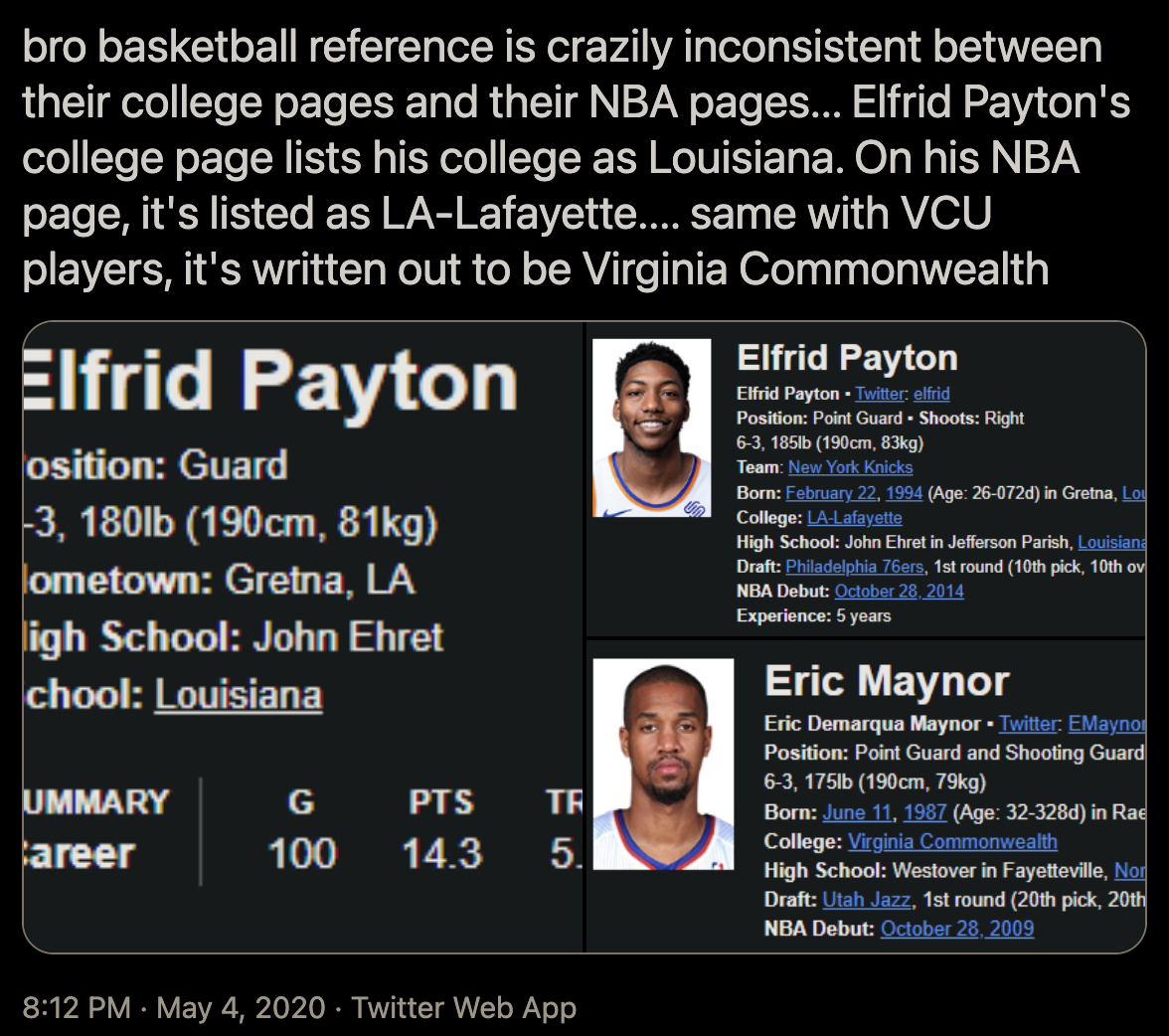
• basketball-reference would spell players' name inconsistently on their own site. For example, basketball-reference had a college page for Patrick Mills but an NBA page for Patty Mills. This isn't super common, but I had to create a dictionary of exceptions for that.
• Same with college names. One page had Louisiana, the other had LA-Lafayette.
• The format of some of the college tables have changed since 2009. Blake Griffin's college basketball-reference page is missing a lot of advanced numbers, along with some of the per-minute ORTG & DRTG numbers. This makes it harder to scrape and it makes the model less accurate, but I'll talk more to that point towards the end.
• Common player names were truly a nightmare. With names like Mike Scott, Gary Clark, and even Anthony Davis, it was difficult to ensure that I landed on the correct player page.

All in all, finding these inconsistencies resulted in me adding ~175 lines of pure Python dictionaries just to map players to the correct pages.

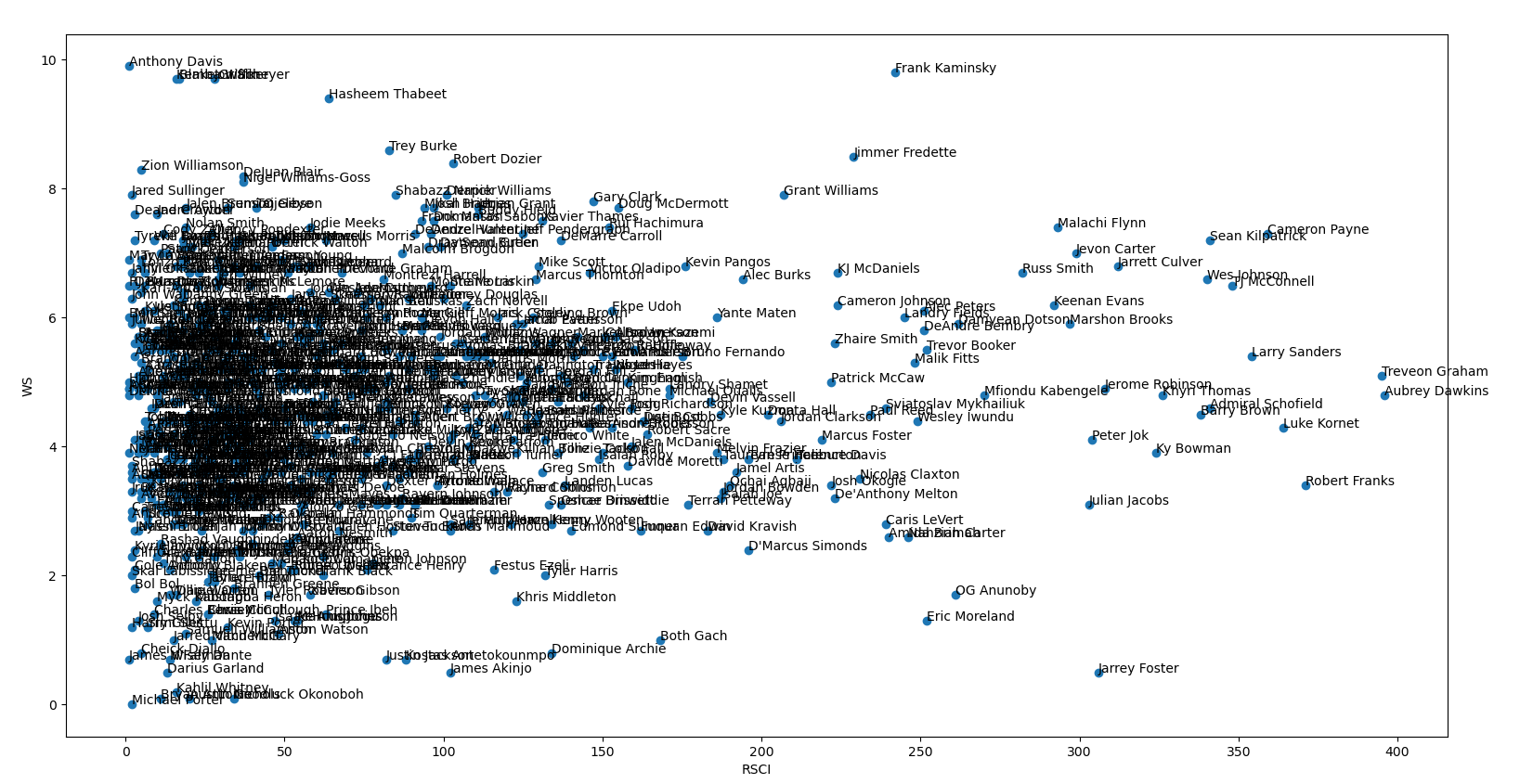
Once I figured out all these exceptions and started scraping the basketball-references pages successfully, I appended all of this data to the pandas DataFrame. Armed with lots of data, Step 3 was to do some preliminary analysis using matplotlib. I wrote some basic scatter plot functionality with two stats along the axes. Below, I graphed high school recruiting rankings by college win shares to see if there was any clear visual indication that higher recruits lead to more wins.

For Step 4, I actually get to start training the machine learning models. Now, just as a disclaimer, I learned everything I've known about machine learning through this project. I have never taken an ML class or done any other project in this field, so a lot of this was my best guess.

In order to get the model ready, there's a lot I had to do to prep the data.

1. Fill in all the missing advanced stats with average values for the row (which is another potential pitfall with the model)
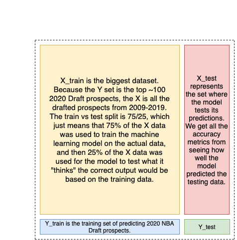
2. Separate the 2020 NBA Draft prospects from the previous NBA Draft prospects. The ~1100 drafted prospects become our X (independent) dataset, and the 2020 prospects become the Y (dependent) dataset. Basically, I use X to predict Y.
3. Come up with a binary classification of an NBA player to tell the model. I came up with a simple algorithm to determine if a prospect was an NBA player based on games & minutes played depending on number of seasons played.
4. Decide what stats to pass in the model to make predictions. I settled on some simple numbers (Height, Years in College) mixed with more advanced stats (ORTG/DRTG, WS, BPM, TS%, AST/TOV, etc) without any traditional box score/counting stats.
5. Most importantly, separate the X dataset into the train and test datasets. After some tinkering (and googling), I settled on 75/25 as the train/test split as that seemed to align with better accuracy for both models. The picture below explains what that means in greater detail.

Now, onto the models. The first model I experimented with was a simplistic Logistic Regression model from scikit-learn. I passed in two parameters to the constructor, one the changes the solver to liblinear because that is apparently better for smaller datasets, and a higher number of iterations to (hopefully) make the model more accurate.

logreg = LogisticRegression(solver='liblinear', max_iter=500)

After fitting the training data to our liblinear model, I was able to run the model and make some predictions. As you can see in the image below, the model hovered around 70% accuracy with 67% precision.

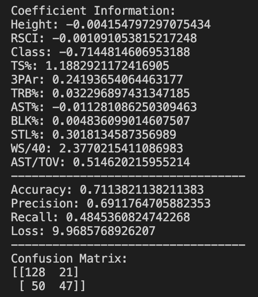
Because the classifications for machine learning models can be a little complex, I'll try to explain what all these metrics mean. The coefficients at the very top of the picture are exactly as they sound: coefficients for each variable that lead to the results. That means for this version of the model, Win Shares/40 (WS/40) were positively correlated with a successful NBA career, and Class (Freshman, Sophomore, etc.) was negatively correlated.

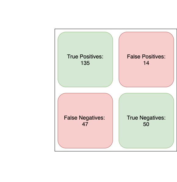
To contextualize some of these numbers, 70.3% accuracy simply means that 70.3 of the predictions made by the model were correct. In the image below, I show the formula as (TP + TN) / Total. This is just True Positive predictions (players the model predicted to be in the NBA that actually were) + True Negative predictions (players the model correctly predicted weren't NBA players) divided by the total number of predictions made. Recall and Precision are described similarly in the picture.

Loss, to my best understanding from reading this stackoverflow answer, is just a summation of the errors made in the training set. I don't know what exactly defines an error, but I know that the goal is to reduce loss for the model.

The confusion matrix is best described through the picture above. Basically, it's just a simple visual classification of the results of the prediction.

That wraps up the explanation of the logistic regression model. Tensorflow is a more complex machine learning algorithm that defines and trains neural networks. A neural network is basically a machine learning model that creates and utilizes nodes in a way similar to a brain's neurons. Because the tensorflow model is very different than the simpler regression model, I need to normalize the data in the way the model can understand it.

normed_x_train = normalize(x_train, x_train.describe().transpose())
normed_x_test = normalize(x_test, x_test.describe().transpose())

What the above code snippet does, to my best understanding, is make the data more meaningful. Normalization gives the model context it wouldn't have otherwise. For example, the low/high-ends of True Shooting % of these prospects are 40% and 80%, respectively, whereas other stats like Offensive Rating, are between 80-120. This makes it extremely difficult for a good model to sensibly understand the nuance with those numbers if you don't normalize the data and compare it to the standard deviation/mean.

def normalize(val, stats):
    val = (val - stats['mean']) / stats['std']
    return val

The stats are now officially in a good place. Setting up the model is equally difficult. I'll describe what the below picture means as best as I can.

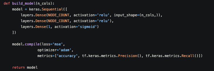
• Keras is a deep learning API that runs with Tensorflow. Here, I am using keras.Sequential to group a linear stack of layers. Honestly, I'm still not exactly sure what that means, but it seemed like it was the easiest to setup.
• NODE_COUNT is a constant here that is equal to 32. I am creating two layers of 32 nodes because that's what I found worked best for the model through some Google searches and experimentation. The last layer is just the output layer. The node layers work autonomously as perform some computation on whatever information is inputted into the node, and then they output to a node in the next layer.
• The parameters are equally confusing. relu activation means.... I'm not sure honestly. It was just by far the most popular activation parameter for Keras layers. Sigmoid activation, on the other hand, is an easy way to pipe the output to one value between 0-1.
• The compilation of the model just outputs the desired metrics. The loss parameter stands for "Mean Squared Error," which is the default way to ouput the loss metric. The optimizer parameter of adam was chosen because it works well with little tuning of the parameters of the model. Finally, I add in the output metrics I care about.

After clarifying the model, I have to choose how many iterations the model will run for. If you recall, I ran the logistic regression model for 5000 iterations. With tensorflow, I choose 50 iterations. This is because if you run the tensorflow model for too many iterations, you risk over-fitting the model. This means that the model gets more accurate on the training data, but less accurate for its predictions on the test data.

And now, to the tensorflow metrics.

Okay, the results are pretty clear to me... the tensorflow neural network model is predictably performing better than the logistic regression model. There isn't a significant difference, but this is good. This means I most likely didn't screw up somewhere along the way running the tensorflow model.

One more model - Gradient Boosting Machines. I learned about GBMs from researching algorithmic stock trading, as GBM models consistently win amateur algo trading competitions. I don't know much about how they work, I just know that they function as essentially multiple sets of decision nodes. At each node, it makes a simple yes or no decision based on certain stats, and does this for a lot of nodes. This is called a decision tree. After multiple iterations of making decision trees, the model eventually comes to find out the best, most accurate model based on the results.

GBMs are just iterative, complex versions of decision trees. The code is rather simple without too many confusing parameters, so I don't think it's necessary to dive into it. With that being said, how does it compare to the neural network and logistic regression models?

This is a little bit shocking to me. Despite the lower accuracy, GBM leads to higher precision and recall metrics. Also, considering this was the simplest to setup with scikit-learn, I can definitely see the appeal for gradient boosting models.

So the metrics are clear. Now who specifically did the models like?

In order to get a clear picture, I ran the 3 models 10 times each. I added up the scores given to each 2021 prospect through all runs to create one singular score for the models. The top 5 is below.

1. Jaden Springer - 24.8
2. Scottie Barnes - 24.3
3. Cade Cunningham - 24.2
4. Jalen Suggs - 24.1
5. Evan Mobley - 23.7

Wow that's a pretty accurate list! Sure, Springer & Barnes aren't usually considered to be top 5 material, but the model recognized Cade, Suggs, and Mobley having incredible freshman seasons.

The next few guys are a little wonky (Drew Timme, DayRon Sharpe, and Mark Williams), but let's ignore that because it doesn't fit my narrative!

Some other notables were Franz Wagner (13th), Corey Kispert (39th), and James Bouknight (69th).

Your models did pretty well! How can you continue to improve them?

I’m glad you asked! There’s a LOT that can be improved. Here are three ideas I have been toying around with recently:

1. Support more stats. Replacing true age rather than years in college would probably reflect potential a little bit better. Wingspan would also be a big help with contextualizing some prospect profiles. Maybe even figure out how to pull in RAPTOR?
2. Increase sample size. Sadly, this isn’t something I can feasibly do, but adding more prospects year after year will make the model more accurate.
3. Try to hypertune some of the data in the columns. For example, I think the models could benefit from looking primarily at height first, and then basing it's conclusion on the height. I think, generally speaking, the models objectively consider a 6 foot player to be the same as a 7 foot player without understanding the positional nuance. Not sure if that's something I can change, but I could look into it.

So that’s all I got. All the code I wrote can be found here if you want to dive in. I am VERY open to hearing feedback if anyone has any. I know there’s a lot of work I can do to improve this model, but I don’t think I will right now. I’m happy with all the knowledge I’ve gained.

I hope I lived up to my self-proclaimed billing on an NBA Draft guru.

Thanks for reading!